Digital Magic vs. The
Jitter
Bug
On Removing the "Shakes" from
Video
Imagery of the 23 November 2003 TSE from QF 2901
Glenn Schneider, Steward
Observatory,
University of Arizona
THE BOTTOM LINE FIRST:
23 November 2003 Total Solar Eclipse
 Raw Video Acquired by: Jay Friedland
Digital Image Processing and Composition
by:
Glenn Schneider
Raw Video Acquired by: Jay Friedland
Digital Image Processing and Composition
by:
Glenn Schneider |
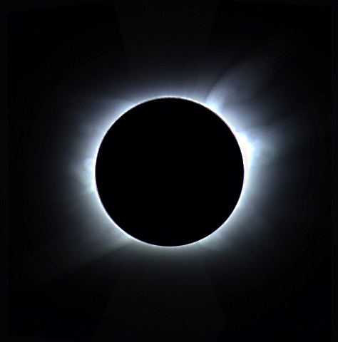
Post-Composition Spatial
Filtering
Click HERE for an
explaination of process.
|
and now... for the rest of
the
story...
THE PROBLEM:
On the QF 2901 Antarctic
eclipse flight many people recorded totality with hand-held
video cameras with relatively high optical magnifications resulting in
"the shakes" of varying levels of degree. The "shakes" cause both
intra-frame image smear, and inter-frame image displacement (loss of
registration).
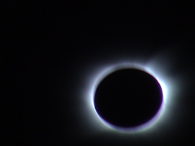
As an example, here are a couple of frames from a representative 15
second
segment of a Digital Video (30 Hz frame rate) taken by Jay Friedland
(one
of my collaborators on our TSE 2003 imaging program):
To get a better, dynamic, feeling of this, it
really is best to VIEW THE RAW
VIDEO
SEGMENT. It's 53 Mbytes, which is why it is just a 15 second
extract, but this should be seen to set the context for the rest of
this
discussion . If it doesn't display in your web browser then download
the
file and view it with a stand-alone QuickTime viewer. Get a QuickTime
viewer from Apple if you don't have one, even Windoze folks.
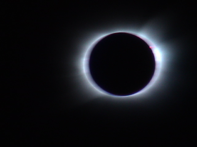
Every once an a while, though, an individual
frame
is steady enough so that in isolation it is quite usable. Such as
this one:
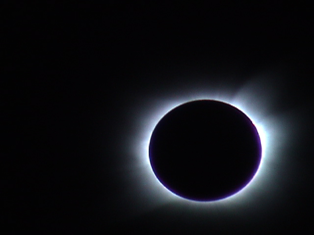
Before going on, a slight digression. If
the lunar disk seems flattened in the above images, it is, but it is an
artifact. Jay had rendered this for Digital Video display, so it
appears "squashed" here. Not an issue, but thought I should
mention
it before someone asked. We can deal with that later.
THE GOAL:
What one really wants to do, first, is isolate
the "good" frames, noting exactly where in temporal sequence they
occur.
The selected frames can then be used in down-stream processing to make
composite images, or re-create a time-correlated video without the
shakes.
The problem is that the "good" frames are comparatively few and far
between.
Video is recorded at 30 frames per second, so for a 2 minute and 30
second
eclipse that would be a lot of frames to pick through and extract
one-by-one.
So, an automated algorithm for Good Frame Extraction (GFE) would be
extremely
helpful. Here, I describe the one I had decided upon and
implemented,
and you can decide how well (or poorly) it works.
THE GFE SOLUTION:
As a matter of practicality, I find it easiest
to work with an image sequence, where each frame is a separate
file.
This is easily done in QuickTime, as exportation of an input movie,
with
frame by frame output as a monotonic sequence of individual image files
(as TIFF, JPEG, PICT, etc.), is accomplished at the push of a
button.
From here on, when I discuss the algorithmic processing of the video
images,
I am actually talking about working through a stack of time-ordered (at
30 Hz rate) individual image files.
First, one needs to decide what the criterion
is to consider a frame "good", and that is wholly subjective.
Clearly,
to declare a frame good it must be "sharp", and the image scene of
interest
(i.e., the full extent of the corona) should not be cut off by the edge
of the frame. But how do you quantify sharpness?
Fortunately,
for THIS application, the lunar limb, seen in silhouette against the
bright
inner corona, provides a natural high-contrast gradient edge on the
close-order
spatial scale of about a pixel. "Sharpness" can be defined in
terms
of the steepness of the radial intensity gradients at the limb
crossing.
Clearly, this will depend upon the intrinsic brightness of the inner
corona,
and also the direction of image smear. In image space this could
be assessed on the azimuthal average (or median), though this would
first
require an edge-location and/or image centroid procedure. This
could
be done, but for images which are smeared this is a difficult
problem.
I first tried this via cross-correlation against an "expected" two
dimensional
edge profile. That worked most of the time, but this approach was
not immune from degeneracies. I am not saying that if pursued more
diligently
that might not work, but I adopted what I feel is a simpler and more
objective
approach.
As another matter of practicality,
quantitative
image processing (which I summarize below) is not actually done
simultaneously
on polychromatic multi-plane images (at least not by me). So each
image was actually first color separated into Red, Green, and Blue
component
images, as separate files. (Working Note: the original conversion
of the DV to an image sequence was into TIFF format, where R, G, and B
information were reformatted into separate files in IDL).
All images were Fourier transformed (two
dimensionally)
and 2D (U/V plane) power spectral images were created (also in
IDL).
The coherent near pixel-scale sharp limb (i.e., in an image without the
shakes) gives rise to a very significant (large amplitude) and
distinctive
high frequency power peak in the power spectrum. There are also
some
large amplitude low frequency components, but those are due to the
large
scale structure of the corona and were ignored (by high pass filtering
of the spectra) (Working Note: Also, the image frame boundaries
were
spatially extended, then apodized with a Gaussian edge profile to
suppress
high frequency ringing.) To identify, quantitatively, what in the
Fourier
power domain this signature looked like, I picked out a few, what
I judged to be, very sharp images. This in itself is somewhat
subjective,
but the eye/brain system makes a pretty good image processor - but I
wouldn't
want to do that for many thousands of frames. I then averaged
their
power spectra and used that as a "training spectrum" against which all
others were compared. (Working Note: This comparison was done
only
on the "green" images, which offered the highest signal-to-noise
without
any image saturation.), In doing the comparison I parametrized a
"good" fit as having its primary high frequency power peak (and its
first
two harmonics) within +/- X% of the frequency of that in the training
spectrum,
and (once identified) normalized amplitudes within +/- Y%.
THE RESULTS:
X and Y, above were determined empirically
(more
subjectivity), and empirically by re-running the above GFE
procedure.
With X and/or Y small, only a very small number of frames were
selected.
Those which were, were very sharp when examined, but were few. If
X and/or Y are more generously broad then more frames are selected, but
at
the expense of decreasing sharpness. In the end, WITH
THESE
DATA, I compromised on X = 20% and Y = 5%. I believe the
fairly
small intensity filter for Y works only because every fame was exposed
identically (and there are no worries about differential
non-linearities
or significant saturation effects in this particular set of images).
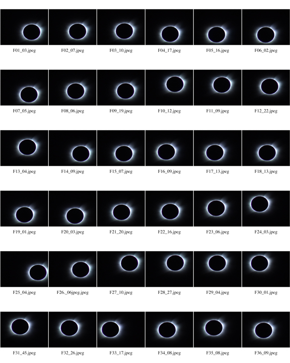
So... what did I get from the 900 input frames
in this 15 second piece of Jay's video? Thirty-six (36) "good" frames
by
the above metric and selection criterion. The equivalence to the
same number of frames in a 35mm roll of film is PURELY a
coincidence!
HONEST! And, what was selected? The R, G, B images of the
selected
frames were recombined into color images, and are shown below (in
reduced
size). When you look at that, you really should again view the
input
video, and scan through that frame-by-frame. See if you
agree.
Then think about doing that (and the marking and extraction) manually
for
the 4500 frames from Contact II to contact III.
Here are the selected frames (in a reduced
size
gallery).
Click on the gallery image itself to see that
at 2x the in-line image size.
Or, you can see the "full
size" images (rendered as JPEG for web viewing).
The file names identify the order of the
frames
(F01, F02...) but also indicate how many frames (1/30th second per
frame)
were REJECTED before the next sequentially selected frame (you
should
see some of the rejections [please do] - I'm sure Jay's dancing for joy
was responsible for some of that jitter). This information (the
timing,
not Jay's dancing) is important in order to maintain the absolute
chronology
of the selected image sequence.
ADDITIONAL PROCESSING - IMAGE
REGISTRATION:
Upon detailed inspection of the full size
images,
you will note that some are sharper than others. And, of course,
the selected images are located all over the field-of-view. These
selected images were edge-padded (with black), stacked, and
registered.
The green color separated images were used to determine the
differential
offsets, and those same determined offsets applied to the corresponding
R and B frames. The registration was done in IDL, using IDP3* as
follows:
| * All quantitative image processing was
performed
using IDP3
(an IDL based image analysis package developed by the NICMOS IDT for
processing Hubble
Space
Telescope imaging data) and algorithms also developed and tested in
with TRANSFORM (a quantitative image data visualization application
under NoeSYS by
RSI, a Kodak
company) and APL X
for Macintosh (MicroAPL Ltd, UK). subsequent image compositing
and
rendering was done with Adobe Photoshop 7.0. Did I say it's all
on
a Mac? I didn't? It is. |
a) The images were geometrically
corrected
for the elongated DV aspect ratio to circularize the lunar disk.
Geometrical correction was accomplished by resampling the images via
bi-cubic
interpolation apodized by an apodizing sync function on a rectangular
pixel
grid.
b) Images were also sub-pixel shifted by
bi-cubic sinc function apodized interpolation, to a common position
actually
(a) and (b) in one step to minimize interpolation errors.
c) Initially, image F01 was shifted (as
described in B) to the center of the output field of view.
d) Registration was accomplished by
sequentially
differencing images and minimizing the subtraction residuals in the
corona
at a zonal radius from 1.05 R(sun) to 1.2 R(sun). This provided a
near optimum region, in terms of S/N for difference minimized
registration.
Note: Registration was NOT done to the lunar disk, as it was moving
across
the Sun.
Note: At this point I had not corrected for
image
ROTATION, which is apparent at the level of about a degree or two,
differentially,
through the image stack over timescsales of many seconds. This
effected
the efficacy of the image registration. However, the residual
image
blurring (which resembles defocus) had the most pronounced effect on
the
precision of the image registration.
So... Here are the REGISTERED selected images:
Click on the gallery image itself to see that
at 2x the in-line image size.
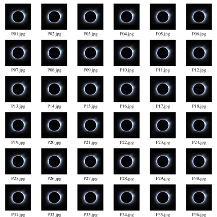
Or, you can see the "full
size" images (rendered as JPEG for web viewing).
This image sequence is also assembled as a QUICKTIME
MOVIE (23 Mbytes). This movie is NOT at the real-time frame
cadence
of the "good" input frames, but is presented at a fixed rate of 2
frames
per second. This allows for easy comparative scanning through the
images.
The inter-frame gaps can be, instead,
interpolated
and filled to produce a smooth real-time movie. I haven't done
that
yet, but it is on the list.
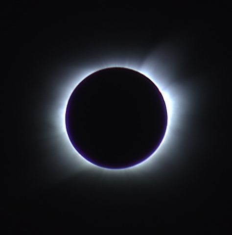
ADDITIONAL PROCESSING - IMAGE
COMBINATION:
A number of the individual images, however,
while
selected to allow the construction of a video are, subjectively, still
a bit too soft due to residual image motion to be used optimally in an
image combination. So, the GFE algorithm was re-run with a bit
more
stringent selection criteria in frequency and amplitude and 11 images
were
rejected previously selected were rejected. The frames then
selected
correspond to images numbers 01, 02, 03, 04, 05, 06, 08, 11, 12, 13,
14,
15, 17, 18, 19, 20, 21, 22, 23, 24, 25, 26, 31, 32, 33 from the above
gallery.
The stacks of corresponding R, G and B images were median collapsed,
and
color combined - linearly - to produce the image at the top of the page.
The component images, however have small
ROTATIONAL
mis-alignments, so are being taken out out, by the same sequential
difference
minimization process as the transitional offsets., even as I write this
and should (I think) produce more structural detail in the
corona.
I will also do weighted radial median filtering with those images to
better
sample the full dynamic range captured by the final stack of
images.
This (and other) images are in work, so check back in a few days.
I *JUST* saw an email from Jay F. (hi, Jay)
informing
me that he has electronically transferred the rest of the video
segments.
Eventually ALL will be processed in the manner discussed here, or
perhaps
with better ideas as they may evolve over time. Stay tuned.
Cheers,
-Glenn Schneider-